Four ppm measurement of the antihydrogen ground-state hyperfine splitting

The observation of hyperfine structure in atomic hydrogen and the high-precision measurements of its zero-field ground-state splitting, at the level of seven parts in 10¹³ (1 mHz absolute uncertainty)^11,18,19, were landmark achievements. These results provided the first evidence of the anomalous magnetic moment and advanced quantum electrodynamics of the electron. In antihydrogen, measurement of the ground-state hyperfine splitting offers a powerful test of CPT symmetry, complementary to comparison of the 1S–2S transition frequencies measured with Doppler-free two-photon spectroscopy²⁰. The hyperfine splitting frequency is a particularly sensitive probe of the internal structure of the antiproton through the Zemach correction and nuclear polarizability at the level of 40 parts per million (ppm) (refs. ^16,21). Recently, the 2S hyperfine splitting of antihydrogen was inferred by combining laser spectroscopy of the 1S–2S transition with our previous determination of the ground-state hyperfine splitting¹⁴. However, the precision was strongly limited by the latter. Finally, precision measurements of the 2S and 1S hyperfine splittings can be combined to determine an experimental value for the Sternheim interval²² in antihydrogen, \((8{a}_{2{\rm{S}}}-{a}_{1{\rm{S}}})/h\), which is largely insensitive to nuclear-structure effects and provides a means to probe high-order quantum electrodynamic (QED) effects¹⁶.

Our experiments are conducted at the CERN Antiproton Decelerator facility using the previously described ALPHA-2 antihydrogen apparatus²³. Key elements of this device are shown in Fig. 1a. Antiproton (\(\overline{{\rm{p}}}\)) and positron (e⁺) plasmas held in a cylindrical Penning–Malmberg trap²⁴ are cooled, radially compressed and merged to synthesize antihydrogen. The latter occurs in a 0.54-K-deep magnetic potential well, in which (neutral) anti-atoms in appropriate spin states and with sufficiently low kinetic energy are confined; that is, they are prevented from interacting with the (matter) surfaces of the apparatus and annihilating. A typical antihydrogen production sequence lasts about 4 min and yields about 100 trapped anti-atoms. This number represents a marked improvement over previous antihydrogen measurements and results from the substantial decrease in positron plasma temperatures achieved by sympathetically cooling the e⁺ with laser-cooled beryllium ions¹⁷. This production process can be repeated many times without releasing anti-atoms²⁵. In this way, we accumulate samples of roughly 1,500 atoms from consecutive cycles over approximately 1 h.

The alternative text for this image may have been generated using AI.

Full size image

a, Cross-sectional schematic of the ALPHA-2 apparatus, including magnets, Penning–Malmberg trap electrodes, annihilation detector and microwave injection system (μ-waves). Antiprotons (\(\bar{{\rm{p}}}\)) and positrons (e⁺) are injected from opposite ends of the apparatus, and the two solenoids in the preparation areas aid in cooling and compression of the charged particles. The 1 T external solenoid surrounding the trap is not shown. b, Calculated magnetic field profile along the trap axis.

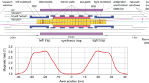
The on-axis magnetic trapping potential for anti-atoms is shown in Fig. 1b. It is formed by the superposition of magnetic fields produced by currents in several superconducting coils in a common cryostat: an octupole, five short solenoids or ‘mirror coils’ and two longer, end solenoids. An external superconducting solenoid surrounds the atom trap and provides a uniform 1 T field for charged-particle confinement. The octupole provides radial \(\bar{H}\) confinement; the two outermost mirror coils provide axial \(\bar{H}\) confinement; and the end solenoids aid in cooling and compression of charged particles. The three remaining mirror coils are used to shape the magnetic field for spectroscopy (see below). Currents in the octupole, solenoids and mirror coils are actively controlled and stabilized using feedback from direct current current transformers (DCCTs). The current in the external solenoid is set to a target value, and the magnet is then disconnected from its power supply while current continues to flow in the superconductor (persistent current mode). Microwaves are injected into the apparatus through a custom-built vacuum window and propagate down a waveguide to the trapping region. Antihydrogen annihilation events are monitored by tracking the trajectories of antiproton annihilation products (charged pions) through a three-layer silicon vertex detector (SVD) with approximately 3π solid-angle coverage of the trap midpoint^23,26 (Methods).

The positronic ground state of antihydrogen is split into four hyperfine sublevels that we denote as |a⟩, |b⟩, |c⟩ and |d⟩, in order of increasing energy in weak magnetic fields (Fig. 2a). Anti-atoms in states |c⟩ and |d⟩ are low-field seekers and can be trapped in the vicinity of a magnetic minimum; anti-atoms in states |a⟩ and |b⟩ are high-field seekers and are rapidly ejected from our trap and annihilate on the surrounding surfaces. The current experiment uses microwaves at frequencies between 28 GHz and 31 GHz to resonantly and sequentially drive the positron spin-flip transitions |c⟩ → |b⟩ and |d⟩ → |a⟩. Near 1 T, the transition frequencies depend approximately linearly on the magnetic field strength with a slope of 28 GHz T^–1. The highly inhomogeneous magnetic field of our trap, with a depth of 0.8 T (set by the radial confining field), results in a strong positional dependence of the resonant frequencies. We therefore tailor the field to be as flat as possible, while ensuring the existence of a shallow centrally located axial field minimum (Methods and Extended Data Fig. 1) and focus on inducing transitions at the minimum of the magnetic potential. First, the |c⟩ → |b⟩ transition is driven at a monotonically increasing frequency, f_cb, in the form of a staircase function, until all |c⟩-state anti-atoms are nominally eliminated, at which point the |d⟩ → |a⟩ transition is driven in the same manner at a frequency f_da > f_cb (Fig. 2b). For each transition, we look for the onset of annihilation events as anti-atoms traversing the absolute minimum in the magnetic potential are brought into resonance. To the extent that the minimum magnetic field is the same for both transitions, and assuming the Breit–Rabi diagram for ground-state antihydrogen is analogous in structure to that of hydrogen, the corresponding frequency difference f_da(B_min) − f_cb(B_min) is equal to the antihydrogen hyperfine splitting frequency a_1S/h (Methods). Note that the order in which transitions are driven cannot be reversed (that is, |d⟩ → |a⟩ followed by |c⟩ → |b⟩) because |c⟩-state atoms at high magnetic fields will come into resonance when driving |d⟩ → |a⟩ transitions near the magnetic minimum. This will remove |c⟩-state atoms from the trap and create a high annihilation background that will mask the onset of |d⟩-state atom annihilations. Similarly, we must scan from low to high frequencies for each transition to obtain a clear annihilation signal when the resonances at the magnetic minimum are reached.

The alternative text for this image may have been generated using AI.

Full size image

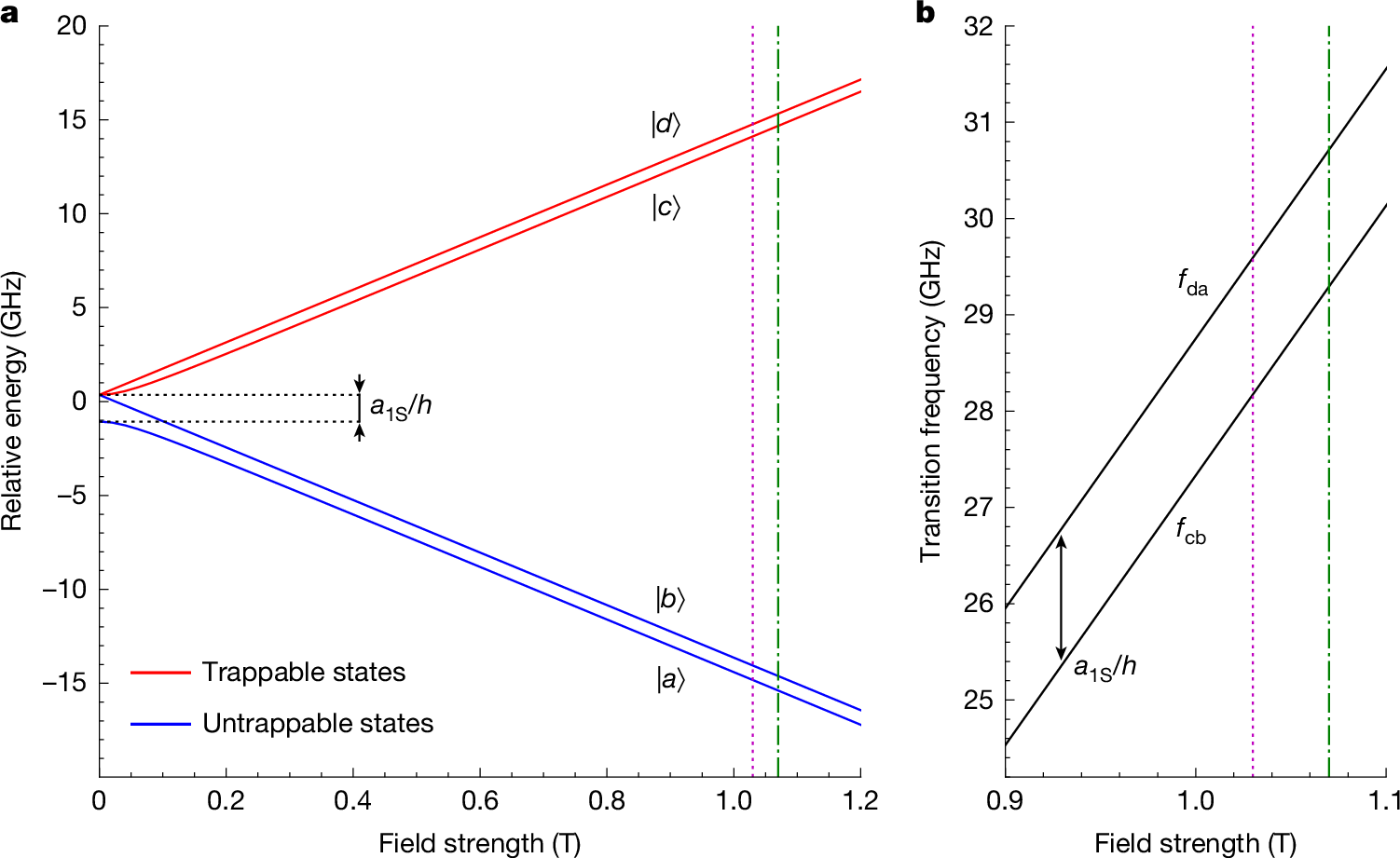
a, Relative energies of the four hyperfine sublevels of antihydrogen’s ground state as a function of magnetic field strength. The dotted purple line and dot-dashed green line indicate the axial magnetic minimum fields (1.03 T and 1.07 T), in which the two spectroscopy experiments were performed. b, Frequencies of the two positron spin-flip transitions used for spectroscopy |d⟩ ↔ |a⟩ and |c⟩ ↔ |b⟩ as a function of magnetic field strength. Frequencies are calculated assuming the properties of antihydrogen mirror those of hydrogen.

We performed two hyperfine splitting experiments at two different base magnetic fields by changing the current in the external solenoid. In both experiments, the magnetic trap shape is maintained, but the first has an on-axis magnetic minimum of 1.03 T and the second of 1.07 T, which corresponds to a 1.1 GHz shift in transition frequencies. In each experiment, the external solenoid is set to the target current and then put into persistent current mode. We then energize the trap magnets to a fixed and stabilized current to create the flattened magnetic trap for the remainder of the experiment. Following this ramp, we observe the minimum magnetic field strength initially rise, level off and then enter a linear decay region, reducing the frequency of the positron spin-flip transitions by roughly 74 kHz per hour for the remainder of the experiment (Methods). We attribute these drifts to fine-scale flux redistribution in the superconductors of the trap magnets, combined with the decay of the persistent current of the external solenoid. After the trapping magnets are energized, we wait a minimum of 1.5 h before beginning spectroscopic experiments to ensure the magnetic field evolution is in the linear decay region.

Both hyperfine splitting experiments consist of eight replicates that characterize the |c⟩ → |b⟩ and |d⟩ → |a⟩ resonances at the magnetic minimum. Each replicate begins with the accumulation of roughly 1,500 antihydrogen atoms from repeated positron–antiproton mixing cycles executed over a period of approximately 1 h. After each mixing cycle, pulsed electric fields are applied to eject any remaining charged particles. Microwaves are then introduced in four phases. Phase 1 involves a 48-step frequency staircase, with a step size of \(\Delta f=5\,\mathrm{kHz}\) and a step duration of \({T}_{s}=8\,{\rm{s}}\). We start Phase 1 roughly 100 kHz below the expected |c⟩ → |b⟩ resonance and scan 240 kHz to characterize the resonance at the magnetic minimum. After Phase 1 we observe that some \(|c\rangle \)-state anti-atoms remain in the trap, which we attribute to anti-atoms on orbits that did not come into resonance near the magnetic minimum. Left in the trap, these anti-atoms would present an increased annihilation background when characterizing the |d⟩ → |a⟩ resonance. Phase 2 removes these |c⟩-state anti-atoms with a 16-step frequency staircase, with the same step size and duration as Phase 1 but roughly 1 MHz below the expected |d⟩ → |a⟩ resonance. This higher frequency range increases the size of the resonant volume and is observed to effectively remove the remaining |c⟩-state anti-atoms. The microwave field slightly heats the trap electrodes so following Phase 2 the microwave drive is switched off for 300 s to allow them to cool. Heating of the trap electrodes will increase the rate of outgassing and could result in a higher rate of antihydrogen annihilations on background gas during phases 3 and 4. Phase 3 is identical to Phase 1 except that the frequency at every step is higher by 1,420,390 kHz (corresponding to the hyperfine splitting for hydrogen minus the expected magnetic field drift), thus probing the |d⟩ → |a⟩ transition. Finally, Phase 4 removes the remaining |d⟩-state anti-atoms by injecting frequencies high above the minimum |d⟩ → |a⟩ resonance. This ensures that there are no residual |d⟩-state anti-atoms in the trap when the next replicate begins.

We track the magnetic field drift by systematically decrementing the frequency at which each subsequent frequency staircase begins, such that the atoms are ejected in the middle of the spectroscopy windows. Owing to the complex electromagnetic environment, the spatial microwave field structure inside the trap is not well understood and changes with frequency; hence, we choose the injected microwave powers in phases 1 and 3 to balance the positron spin-flip rates observed in a set of auxiliary experiments (Methods). In each experiment, the overall number of annihilations from ejected |c⟩-state atoms was consistent with the number of events from ejected |d⟩-state atoms. This indicates that equal numbers of |c⟩-state and |d⟩-state are produced and trapped and that the positron spin-flip rates for each transition are roughly equal.

The annihilation of ejected \(\bar{H}\) detected by the SVD during Phase 1 and Phase 3 of each replicate yields resonance lineshapes for the |c⟩ → |b⟩ and |d⟩ → |a⟩ transitions, respectively (Fig. 3). The lineshapes reflect contributions from the structure of the non-uniform magnetic field, the depletion of the antihydrogen population as the microwave frequency is incremented, the orbits of the atoms through the magnetic field, the local amplitude of the microwave magnetic field seen by the atoms, and motional broadening effects. Without full knowledge of these factors, we cannot develop a precise physical model of the observed lineshapes. Instead, we take the approach of fitting the lineshapes with an empirical model with a frequency parameter (\({f}_{\text{cb}}^{{\rm{o}}}\), \({f}_{\text{da}}^{{\rm{o}}}\)), associated with the onset of annihilation events as anti-atoms traversing the magnetic minimum are brought into resonance (Methods). These parameters are proxies for \({f}_{\text{cb}}({B}_{min})\) and \({f}_{\text{da}}({B}_{min})\), respectively, and share the same property that \({a}_{1{\rm{S}}}/h={f}_{\text{da}}^{{\rm{o}}}-{f}_{\text{cb}}^{{\rm{o}}}\) if measured at the same magnetic field. Alternative frequency parameters and models can also be used to extract a_1S/h. For example, consistent results are obtained using the peak (f_max) of the empirical lineshapes (Methods) rather than the onset. Because we are performing a difference measurement and not extracting absolute frequencies for the individual transitions, systematic effects associated with our choice of model largely cancel and the residual systematics can be quantified (Methods).

The alternative text for this image may have been generated using AI.

Full size image

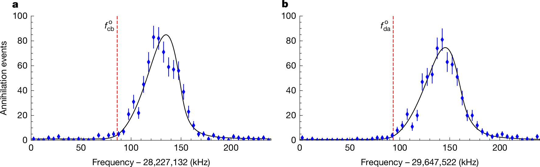
a, An example of the |c⟩ → |b⟩ resonance lineshape obtained by plotting annihilation events against microwave frequency during Phase 1 of a replicate from the 1.03 T experiment. b, The |d⟩ → |a⟩ resonance during Phase 3 of the same replicate. The black lines are the empirical lineshape model, and the vertical red dashed lines indicate the onset frequency parameters, \({f}_{\text{cb}}^{{\rm{o}}}\) and \({f}_{\text{da}}^{{\rm{o}}}\). The error bars represent 1 standard deviation of counting errors.

Because the minimum magnetic field magnitude is decreasing in time, it is different between Phase 1 and Phase 3 (which are separated by 812 s) of each replicate as well as between replicates. To account for this, we assume the magnetic field strength decay is purely linear and fit the two sets of onset parameters with two straight lines with a common slope as shown in Fig. 4. The other two fit parameters are the average of the two intercepts and the separation between the two lines, the latter of which is our estimation of \({a}_{1{\rm{S}}}/h\).

The alternative text for this image may have been generated using AI.

Full size image

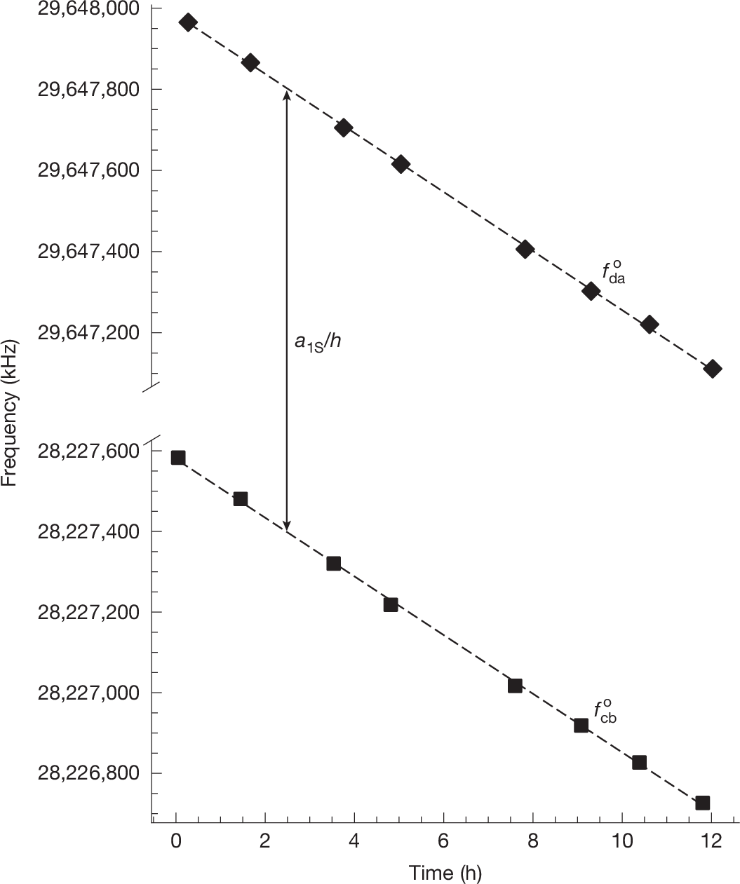
Pairs of onset frequencies are determined from each replicate of the experiment of the 1.03 T experiment. Squares and diamonds denote \({f}_{\text{cb}}^{{\rm{o}}}\) and \({f}_{\text{da}}^{{\rm{o}}}\), respectively, found by fitting the model to the measured resonance lineshape of each replicate. The error bars are not visible on this scale. Dashed lines represent the best-fit linear decay model.

The results for the hyperfine splitting frequencies inferred for the two datasets, collected on separate days at the base magnetic fields of 1.03 T and 1.07 T, are summarized in Table 1, along with statistical and systematic uncertainties (